Solar Prominences
Although the solar corona has been repeatedly observed during total solar eclipses, and remarked about for thousands of years, the next most common solar feature, the prominence, is much rarer. The earliest observation was recorded in the 14th-century Laurentian Chronicle during the solar eclipse of May 1, 1185 CE:
“On the first day of the month of May, on the day of the Saint Prophet Jeremiah, on Wednesday, during the evening service, there was a sign in the Sun. It became very dark, even the stars could be seen; it seemed to men as if everything were green, and the Sun became like a crescent of the Moon, from the horns of which a glow similar to that of red-hot charcoals was emanating. It was terrible to see this sign of the Lord.”
Although there are many petroglyphs and primitive art that show various kinds of protuberances on the solar disk, we cannot be sure what these features were intended to represent by the artists. Instead, we flash-forward to eclipses studied during modern times, especially after 1800 when it became very popular to draw detailed pictures of total solar eclipses for publication in scientific journals and in popular newsprint. The earliest such sketch showing prominences also occurred at the same time that the first daguerreotype photographs were attempted during the eclipse of July 28, 1851. The sketch shown here by French astronomer and politician François Arago actually has greater clarity than the photographs.
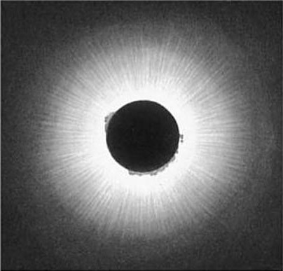
In addition to the magnificent corona there are bright red cloud-like features seen close to the dark limb of the moon. By the May 2, 1733 eclipse, Swedish astronomer Bigerus Vassenius is credited with the ‘ first unequivocal observation of the red prominences” in the Transactions of the Royal Scottish of Arts ( 1856: Vol 4, p 137). It took a few more eclipses before astronomers realized that these ‘maculae’ as some also called them, were not clouds in the lunar atmosphere but were features of the solar atmosphere! Their redness was always a feature associated with their observations, and initially misconstrued as similar to the atmospheric reddening of light near sunset on Earth. Despite studies of these prominences spanning dozens of additional total solar eclipses, real progress in understanding them had to await the advent of the spectroscope and its application by J. Norman Lockyer to their study in 1869. After several failed attempts, he announced in an October 28, 1868 letter to the Philosophical Magazine and Journal of Science, his successful detection of the Fraunhofer C, F and D lines in the light from a prominence. Lockyer also went on to say that “…prominences are merely local aggregations of a gaseous medium which entirely envelopes the sun. The term chromosphere is suggested for this envelope…the spectrum of the chromosphere is always visible in every part of the sun’s periphery.” However, the origin of prominences was still quite the mystery by this time. The development of the spectroheliography at Mount Wilson Observatory by George Ellery Hale in 1906, the solar coronagraph by Bernard Lyot in 1932, and the detection of magnetic fields in prominences by Zirin and Severny in 1961 completely changed our understanding of the origin and evolution of prominences.
It was suspected for a long time that the hydrogen gas detected spectroscopically inside prominences was colder than that of the surrounding chromosphere, and the gas density was near 1011 hydrogen atoms/cm3 far higher than the chromosphere and corona, so some agency must be insulating and shaping them from their environment. It was already known by the early-20th century that magnetic fields were a likely constituent of the solar environment, and the arch-like shapes of prominences resembled iron filings trapped in a toy bar magnet field. Sunspot magnetic fields were detected and measured by George Ellery Hale in 1906 and found to be several thousand Gauss in strength. But the tantalizing prominence magnetism was undetectable until still-more-sensitive techniques were developed and put into practice by Soviet astronomers H. Zirin and A.B. Severny in 1961. They succeeded in detecting prominence fields of 50 Gauss for quiescent prominences and 200 Gauss for active prominences. This led to the modern era of ‘Space Age’ prominence science, which is still unfolding today!
The Prominence Zoo
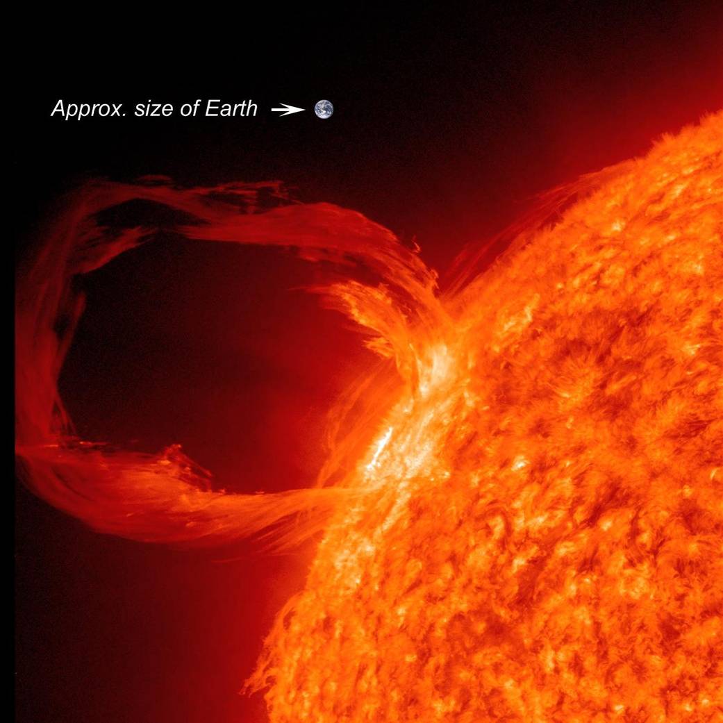
Eruptive Prominences - Here we see a dramatic eruptive prominence imaged by the NASA Solar Dynamics Observatory on March 30, 2010. A prominence consists of two ‘foot points’ on the photosphere, often but not always associated with sunspot regions. The material in a prominence consists of a plasma of ionized gas and neutral hydrogen. The ionized gas interacts with the local magnetic field while the neutral hydrogen is kinetically coupled to the ions and ‘dragged along’. These foot points inject the plasma into local magnetic fields lines, to form the visible prominence whose cooler hydrogen atoms emit in the Ha line that we see during eclipses. Under other circumstances, the plasma inside a prominence can originate in the corona or the chromosphere through condensation. This actually provides a return flow of matter from the hot corona, through condensation into prominences, and then a flow-down onto the photosphere. Most prominences come and go over time scales of months, before they dissipate in a matter of a few hours as eruptive prominences.
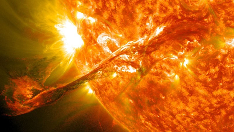
A slightly different view of an eruptive prominence is also obtained by the Solar Dynamics Observatory on August 31, 2012. This view shows that the flowing gas takes complex paths along the twisted field lines in a prominence, and that when the cooler plasma is seen against hotter plasma in the prominence or on the photosphere, it appears darker in contrast.
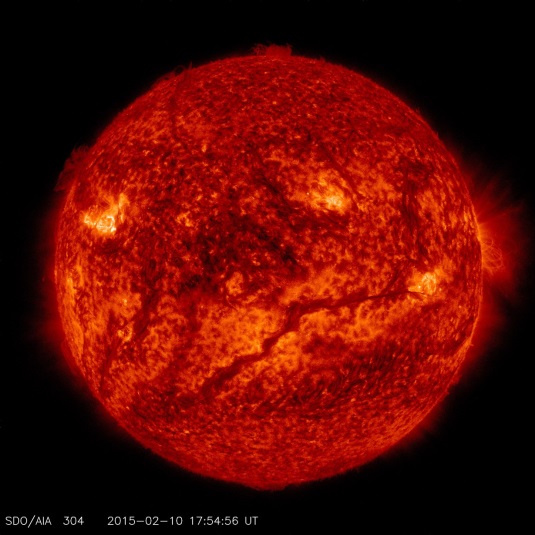
When viewed against the hotter surface of the sun, the cooler material in a prominence looks dark, resulting in a snaking filament of ‘shadow’ across the solar surface. This image was obtained by SDO on February 10, 2015. Even though it appears darker, this is only because it is emitting less light than the background. Taken by itself against the black sky as in the top image, this gas is actually very bright!
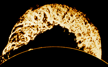
Eruptive prominences represent plasma entrained in a magnetic field but for which the magnetic and thermal pressures are unbalanced compared to the pressure of the external chromospheric and coronal plasma along with the sun’s gravity. The result is that the loop of plasma continues to grow and expand as it reaches greater heights above the photosphere. These expanding loops can also encounter other magnetic loops, and if the lines of force are of opposite polarity, they can reconnect and merge into still-larger magnetic structures that continues to grow and expand, perhaps eventually becoming a coronal mass ejection. One of the largest erupting prominences ever recorded was observed with a coronagraph on June 4, 1946 at Climax, Colorado. On December 19, 1973 Skylab astronauts captured on film another ‘famous’ large eruptive prominence.
A second class of prominences are the quiescent prominences. Like a pencil balanced on its tip, these magneto-plasma structures appear to remain frozen in space for weeks and even months before becoming unstable and becoming erupting prominences. The plasma in these prominences can sometimes be seen draining down from their apex onto the photosphere. Presumably when this process reaches a critical point, the available mass of the remaining plasma is unable to resist the upward magnetic pressure against gravity and the quiescent prominence disperses. A quiescent prominence can also be ‘activated’ into eruptive prominence when a new prominence forms underneath it and bumps into it from below. The delicate balance of magnetic, thermal and gravitational forces is then pushed out of equilibrium, and the whole shebang of plasma and magnetic fields erupts outwards.
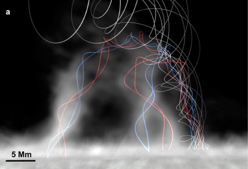
The magnetic fields inside prominences are not the smooth fields we see in toy bar magnets, but are twisted by the turbulent and convective motion of the plasma at the base of the prominence. Here is a representation of a 3D model of magnetic field data obtained by M. J. Martínez González and his colleagues in 2015. Compare this to the image of the 1946 eruptive prominence whose plasma shows a definite helical twistedness to it.
During total solar eclipses lasting only a few minutes, no motion is visible in the prominence shapes typically observed, but thanks to the advent of coronagraphs and spectroheliographs, we can actually create movies of the evolution of prominences at the solar limb even without the benefit of an eclipse! Spacecraft such as the Solar and Heliospheric Observatory (SOHO), the Solar Dynamics Observatory (SDO), Hinode allow unobstructed views of the sun round-the-clock to study at high resolution and cadence all of the complex changes that occur in prominences.
Similar in character to the prominences are coronal loops, but their details are quite different. Coronal loops are often seen above sunspot groups as very fine lines similar to what is produced with iron filings and a toy magnet. The magnetic field lines are smoother than for a prominence, moreover, the plasma filling coronal loops is far-hotter than in a prominence. This means that coronal loops do not emit light from neutral hydrogen atoms, which are now fully ionized, but from the simple thermal emission of the heated plasma at over 100,000 Celsius. Some atoms such as iron still have a complement of electrons that can emit light at discrete wavelengths in this plasma, and these lines are often used to determine the exact temperature and density of coronal loop plasma, such as with the Hinode Extreme Ultraviolet Imaging Spectrometer (EIS) instrument. Coronal loops emit copious amounts of light at extreme ultraviolet and x-ray wavelengths, and are easily studied with instruments tuned to specific short wavelengths where the trapped ions preferentially emit such as the iron lines at 171 Å, 195 Å, 284 Å, and the helium line at 304 Å all used by SOHO, or the additional lines at 1216 Å and 1550 Å from hydrogen and calcium used by the TRACE spacecraft.
High-resolution spacecraft observations such as those by Hinode let us study the coronal loop plasma, from which we can determine average plasma densities of about 109 particles/cm3, and relatively constant temperatures along their lengths. Only about 10% of the actual volume of a coronal loop magnetic tube actually contains emitting plasma so it is mostly an empty structure.
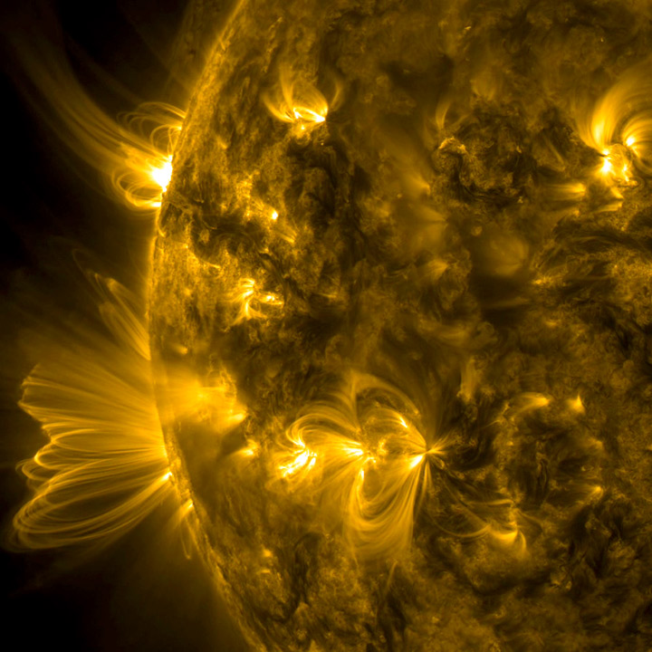
SDO captured a splendid example of expanding coronal loops seen in profile at the edge of the Sun on October 14, 2014. The arcs of the loops we see in extreme ultraviolet light are actually particles spiraling along magnetic field lines arcing above the active region that was the source of the flare. To give a sense of scale, these huge loops are reaching out from the photosphere more than 15 times the size of Earth (100,000 km). (Credit: Solar Dynamics Observatory/NASA).
Coronal loops do not remain static in time. The supply of plasma comes from injection events at the loop’s foot points on the photosphere, which can sometimes be near active regions. These sources move around on the solar surface so loops are constantly ‘turning on’ and ‘turning off’. This effect can be seen in many movies of active regions. The magnetic field lines remain more-or-less fixed while the plasma injection points move, giving the illusion that the magnetic field lines are fanning back and forth or otherwise in motion.
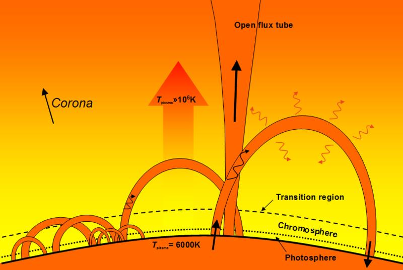
This cartoon shows the different scales of coronal loops that exist in the lower corona and chromosphere. Many scales have been observed and it is believed there are many sub-resolution structures below the transition region threading through the chromosphere. Highly-radiating coronal loops may share the same foot point location as open flux tubes (i.e. solar wind and coronal holes) and therefore may share similar physics leading to the conjecture that coronal loops may share similar heating mechanisms as the solar wind. (Credit: Ian O’Neill, Thesis 2008).